Quickstart: Parsing and Plotting
This example shows the most basic steps to get from a raw BioLector data file to an interactive visualization.
[1]:
import pandas
import ipywidgets
from matplotlib import pyplot, cm

import bletl
In 98 % of the cases, you will use the bletl.parse function to load data.
The function comes with a few arguments that you can use to override calibration settings if your raw data file for example does not specify the correct lot_number.
To learn all about the different options, run help(bletl.parse) or bletl.parse?.
Parsing
In this quickstart, we load a raw data file from the test suite:
[ ]:
bldata = bletl.parse(r"..\..\..\tests\data\BLPro\213-NT_1500rpm_30C_20min--2019-10-18-14-55-15.csv")
# just display the variable containing the data
bldata
BLData(model=BLPro) {
  "BS4": FilterTimeSeries(197 cycles, 48 wells),
  "pH": FilterTimeSeries(197 cycles, 48 wells),
  "DO": FilterTimeSeries(197 cycles, 48 wells),
  "GFP-Gemini": FilterTimeSeries(197 cycles, 48 wells),
  "eYFP - Citrine": FilterTimeSeries(197 cycles, 48 wells),
}
As you can see in the above, the returned BLData object is a dictionary that maps identifiers of filtersets to FilterTimeSeries objects.
Metadata
Additional properties, such as comments, environment or filtersets contain data that is not specific to a well:
[3]:
bldata.filtersets.head()
[3]:
| filter_number | filter_name | filter_id | filter_type | excitation | emission | gain | gain_1 | gain_2 | phase_statistic_sigma | signal_quality_tolerance | reference_gain | reference_value | calibration | emission2 | |
|---|---|---|---|---|---|---|---|---|---|---|---|---|---|---|---|
| 1 | 1 | Biomass4 | 201 | Intensity | None | None | NaN | 4.0 | 1.0 | None | None | NaN | NaN | None | |
| 2 | 2 | pH(HP8) | 202 | pH | None | None | 7.0 | 7.0 | 1.0 | None | None | NaN | 100.000000 | 1924_comp | None |
| 3 | 3 | DO(PSt3) | 203 | DO | None | None | 7.0 | 7.0 | 1.0 | None | None | NaN | 100.000000 | 1924_comp | None |
| 4 | 4 | GFP-Gemini | 204 | Intensity | None | None | NaN | 7.0 | 1.0 | None | None | 3.0 | 135.641129 | None | |
| 5 | 5 | eYFP - Citrine | 215 | Intensity | None | None | NaN | 7.0 | 1.0 | None | None | 6.0 | 160.436661 | None |
[4]:
bldata.environment.head()
[4]:
| cycle | time | temp_setpoint | temp_up | temp_down | temp_water | o2 | co2 | humidity | shaker_setpoint | shaker_actual | |
|---|---|---|---|---|---|---|---|---|---|---|---|
| 5 | 1 | 0.013056 | None | 28.6 | 29.3 | 27.8 | 25.02 | -9999.0 | 76.17 | None | 1500.0 |
| 156 | 1 | 0.076389 | None | 29.9 | 29.9 | 30.4 | 33.20 | -9999.0 | 84.86 | None | 1500.0 |
| 207 | 1 | 0.095833 | None | 29.9 | 29.9 | 31.9 | 34.42 | -9999.0 | 85.36 | None | 1499.0 |
| 285 | 2 | 0.346389 | None | 30.0 | 29.9 | 31.0 | 35.01 | -9999.0 | 85.09 | None | 1499.0 |
| 436 | 2 | 0.409167 | None | 29.9 | 29.9 | 32.9 | 35.10 | -9999.0 | 85.71 | None | 1500.0 |
Accessing and Visualizing Measurements
Depending on what you want to do, you can retrieve measurement data as tuples of Numpy arrays:
bldata.get_timeseriesbldata["pH"].get_timeseries
or as pandas DataFrames:
bldata.get_narrow_databldata.get_unified_narrow_databldata["pH"].get_unified_dataframe
or via the underlying DataFrames that separate time and value:
bldata["pH"].timebldata["pH"].value
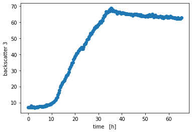
[5]:
# here we retrieve it as numpy arrays, becase that's very convenient for plotting
t, bs = bldata.get_timeseries("BS4", "A02")

pyplot.scatter(t, bs)
pyplot.xlabel('time   [h]')
pyplot.ylabel('backscatter 3')
pyplot.show()
Interactivity
With the ipywidgets package, one can easily create interactive visualizations.
Here, the plotting code from above is wrapped into a plot_one_well function that takes filterset and well as arguments.
The ipywidgets.interact or ipywidgets.interact_manual function is then used to create an interactive visualization, where all the available filtersets/wells are passed as options.
[6]:
def plot_one_well(filterset, well):
    time, value = bldata.get_timeseries(filterset, well)

    fig, ax = pyplot.subplots()
    ax.scatter(time, value)
    ax.set_ylabel(filterset)
    ax.set_xlabel("time   [h]")
    ax.set_title(well)
    pyplot.show()
    return

ipywidgets.interact(
    plot_one_well,
    filterset=list(bldata.keys()),
    well=list(bldata["pH"].time.columns),
);
[6]:
<function __main__.plot_one_well(filterset, well)>
That’s it with the basic tutorial! To learn more about what bletl can do, checkout the other examples.
Also remember to use help(...) and dir(...) to read the attributes/methods/docstrings. They often contain more detailed information than example notebooks.
[7]:
%load_ext watermark
%watermark -n -u -v -iv -w
Last updated: Fri Jul 02 2021

Python implementation: CPython
Python version       : 3.7.9
IPython version      : 7.19.0

pandas    : 1.2.1
bletl     : 1.0.0
matplotlib: 3.3.2
ipywidgets: 7.6.3

Watermark: 2.1.0
[ ]: